Remote sensing offers spatially and temporally continuous measurements of hydrological fluxes like rainfall, evapotranspiration, and soil moisture. These measurements provide valuable information in data-scarce catchments around the world. Nevertheless, owing to a variety of sensor and retrieval algorithms, remote sensing data is subject to large uncertainties and errors. Therefore, it is imperative that remote sensing datasets are rigorously validated using ground truth before such datasets are used for applications such as calibration of climate forecasts, hydrologic modeling, and streamflow forecasting.
As an example, we can compare and validate different remotely sensed precipitation datasets using ground-based measurements for a catchment in East Africa. The area of study is the Omo-Gibe river basin in Ethiopia, using a time period of at least 1 year.
The comparison should focus on:
- Description of catchment climatology using publicly available precipitation datasets
- Preprocessing of these datasets (NetCDF format)
- Comparison of different datasets and
- Validation of these datasets (both spatial and non-spatial).
Preprocessing of Data
First, clear your workspace, set your working directory, and load the required library
# clear workspace
rm(list=ls())
#set working directory
setwd("/home/username/Downloads/Scripts/...")
#load required library
library(raster)
Next, download and preprocess remotely sensed rainfall datasets for the study area.
# load precipitation data
Centrends = brick("CenTrends_v1_monthly.nc",varname = "precip") GPCC=brick("precip.mon.total.v7.nc")
TRMM =brick("prcp_trmm_2004.nc")
# Load Omogibe shapefile
gibe_shp = shapefile("omogibe.shp")
# extract only 2004 data from centrends and gpcc
dates_Centrends = names(Centrends)
dates_GPCC = names(GPCC)
# find year 2004
index_Centrends= grep("2004" ,dates_Centrends)
index_GPCC = grep("2004" ,dates_GPCC)
# subset the data to 2004
Centrends = Centrends[[index_Centrends]]
GPCC = GPCC[[index_GPCC]]
# fix the coordinates of GPCC and TRMM
# rotate gpcc and trmm data, but centrends is correct(no need to rotate)
GPCC = rotate(GPCC)
TRMM = rotate(TRMM)
# crop the datasets to Omogibe catchment
centrends_gibe = crop(Centrends,gibe_shp)
gpcc_gibe = crop(GPCC,gibe_shp)
trmm_gibe = crop(TRMM,gibe_shp)
The datasets include TRMM 3B42RT, CMORPH, PERSIANN, and CenTrends (Ground truth data). Ground truth data (Centrends long-term rainfall record) should be used to quantify the climatology of the study area. Seasonality, inter-annual variability, and long-term change in rainfall in the study area should be adequately described.
Comparison of Remote Sensing Datasets
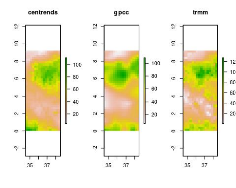
Next, we can complete a comprehensive comparison of the processed rainfall datasets including basin-averaged values and spatial distribution of rainfall in the study catchment for different seasons.
#extract mean value from the 3 datasets
centrends_avg = extract(centrends_gibe,gibe_shp,mean,na.rm=TRUE)
gpcc_avg = extract(gpcc_gibe,gibe_shp,mean,na.rm=TRUE)
trmm_avg = extract(trmm_gibe,gibe_shp,mean,na.rm=TRUE)
# create dataframe of mean values
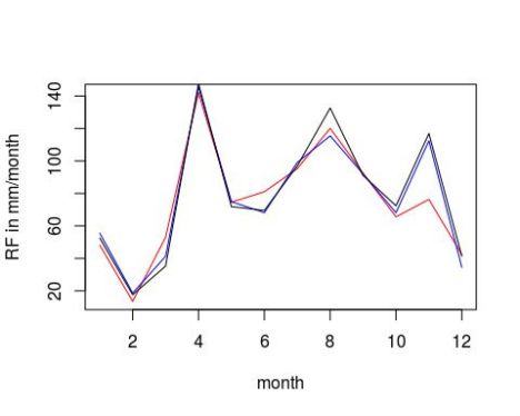
data_mean = data.frame(Centrends = c(centrends_avg), GPCC = c(gpcc_avg), TRMM = c(trmm_avg)) # create a plot of the 3 precipitation data
plot(c(1:12) ,data_mean[ ,"Centrends"],type="l" ,xlab="month" ,ylab="RF in mm/month" ,col="red") lines(data_mean[,"TRMM"],col="blue")
lines(data_mean[,"GPCC"],col="black")

# Comparing raster data (spatially)
# equalize the resolution of the datasets
centrends_gibe = projectRaster(centrends_gibe,trmm_gibe)
gpcc_gibe = projectRaster(gpcc_gibe,trmm_gibe)
# plot three rasters together
# 1=row, 3=columns
par(mfrow = c(1,3))
plot(centrends_gibe[[1]])
title("centrends")
plot(gpcc_gibe[[1]])
title("gpcc")
plot(trmm_gibe[[1]])
title("trmm")
Evaluation of Remote Sensing Datasets
We can calculate relevant error metrics to compare and select the best remote-sensing datasets. While there are many different error metrics, an important one to include is RMSE. Error metrics should be calculated for basin averages and each grid pixel to characterize the spatial distribution of error.
# calculation of RMSE error
GT = data_mean[,"Centrends"] #ground truth
RS = data_mean[,"TRMM"] #remote sensing data
# RMSE
rmse=sqrt(mean((GT-RS)^2))
# calculation of MAE
mae=mean(abs(GT-RS))
# correlation(values varies b/n 1 and -1)
correlation=cor(GT,RS)
# calculation of spatial errors
gt = centrends_gibe
rs = trmm_gibe
# step 1 calculate the dif erence b/n GT and RS data
diff_raster=gt-rs
# step 2 calculate the square of the dif erence
square_raster=(gt-rs)^2
# step 3 calculate the mean
mean_raster=stackApply(square_raster,c(1,1,1,1,1,1,1,1,1,1,1,1),mean,na.rm = TRUE) # step4 calculate rmse for each pixel
rmse_raster=sqrt(mean_raster)
# calculation of of spatial MAE
diff_raster=gt-rs
abs_raster = abs(diff_raster)
mae_raster=stackApply(abs_raster,c(1,1,1,1,1,1,1,1,1,1,1,1),mean,na.rm = TRUE)
Output
# print data and values
centrends_avg
# X2004.01.30 X2004.03.01 X2004.03.30 X2004.04.30 X2004.05.30 X2004.06.30 X2004.07.30 [1,]    48.15352    13.57746    52.95584    141.9959     74.6393    81.02153    95.22529 X2004.08.30 X2004.09.30 X2004.10.30 X2004.11.30 X2004.12.30 [1,]     120.071    92.46025    65.59274    76.29582     42.3984
gpcc_avg
# X2004.01.01 X2004.02.01 X2004.03.01 X2004.04.01 X2004.05.01 X2004.06.01 X2004.07.01 [1,]     52.5218     17.6262     35.2628     147.755      71.842      69.488     96.9292 X2004.08.01 X2004.09.01 X2004.10.01 X2004.11.01 X2004.12.01 [1,]    132.5842     91.0448     72.4016     116.918     41.3116
trmm_avg
# X2004.01.16 X2004.02.15 X2004.03.16 X2004.04.15 X2004.05.16 X2004.06.15 X2004.07.16[1,]     55.5454     18.6204    41.24854    145.4656    74.89386    68.13789    99.03134     X2004.08.16 X2004.09.15 X2004.10.16 X2004.11.15 X2004.12.16 [1,]    115.4681    91.98316    68.13575    112.3921    34.48828
The above results can be summarized in a table and further examined.
- correlation = 0.9402921
- mae = 8.015455
- rmse = 12.25799
| index | index_Centrends | index_GPCC | GT | RS |
|---|---|---|---|---|
| 1 | 1249 | 1237 | 48.15352 | 55.5454 |
| 2 | 1250 | 1238 | 13.57746 | 18.6204 |
| 3 | 1251 | 1239 | 52.95584 | 41.24854 |
| 4 | 1252 | 1240 | 141.99591 | 145.46563 |
| 5 | 1253 | 1241 | 74.6393 | 74.89386 |
| 6 | 1254 | 1242 | 81.02153 | 68.13789 |
| 7 | 1255 | 1243 | 95.22529 | 99.03134 |
| 8 | 1256 | 1244 | 120.07101 | 115.46809 |
| 9 | 1257 | 1245 | 92.46025 | 91.98316 |
| 10 | 1258 | 1246 | 65.59274 | 68.13575 |
| 11 | 1259 | 1247 | 76.29582 | 112.39205 |
| 12 | 1260 | 1248 | 42.3984 | 34.48828 |

