The introduction of the raster package, first developed by Robert J. Hijmans, has been a revolution for geo-processing and analysis using R.
The Raster Objects
The package produces and uses objects of three different classes, the RasterLayer, the RasterStack, and the RasterBrick. A RasterLayer is the equivalent of a single-layer raster, as an R workspace variable. The data themselves, depending on the size of the grid can be loaded in memory or on disk. The same stands for RasterBrick and RasterStack objects, which are the equivalent of multi-layer RasterLayer objects. RasterStack and RasterBrick are very similar, the difference being in the virtual character of the RasterStack. While a RasterBrick has to refer to one multi-layer file or is in itself a multi-layer object with data loaded in memory, a RasterStack may 'virtually' connect several raster objects written to different files or in memory. Processing will be more efficient for a RasterBrick than for a RasterStack, but RasterStack has the advantage of facilitating pixel-based calculations on separate raster layers.
Let's take a look at the structure of these objects.
library(raster)
## Loading required package: sp
## Generate a RasterLayer object
r <- raster(ncol=40, nrow=20)
class(r)
## [1] "RasterLayer"
## attr(,"package")
## [1] "raster"
# Simply typing the object name displays its general properties / metadata
r
## class : RasterLayer
## dimensions : 20, 40, 800 (nrow, ncol, ncell)
## resolution : 9, 9 (x, y)
## extent : -180, 180, -90, 90 (xmin, xmax, ymin, ymax)
## coord. ref. : +proj=longlat +datum=WGS84 +ellps=WGS84 +towgs84=0,0,0
From the metadata displayed above, we can see that the RasterLayer object contains all the properties that geo-data should have; that is to say a projection, an extent, and a pixel resolution. RasterBrick and RasterStack objects can also fairly easily be generated directly in R, as shown in the example below. Being able to generate such objects without reading them from files is particularly important for the generation of reproducible examples.
# Using the previously generated RasterLayer object
# Let's first put some values in the cells of the layer
r[] <- rnorm(n=ncell(r))
# Create a RasterStack object with 3 layers
s <- stack(x=c(r, r*2, r))
# The exact same procedure works for creating a RasterBrick
b <- brick(x=c(r, r*2, r))
# Let's look at the properties of of one of these two objects
b
## class : RasterBrick
## dimensions : 20, 40, 800, 3 (nrow, ncol, ncell, nlayers)
## resolution : 9, 9 (x, y)
## extent : -180, 180, -90, 90 (xmin, xmax, ymin, ymax)
## coord. ref. : +proj=longlat +datum=WGS84 +ellps=WGS84 +towgs84=0,0,0
## data source : in memory
## names : layer.1, layer.2, layer.3
## min values : -3.674132, -7.348263, -3.674132
## max values : 2.854998, 5.709995, 2.854998
The RasterBrick metadata displayed above is mostly similar to what we saw earlier for the RasterLayer object, with the exception that these are multi-layer objects.
Object Manipulation
The actual data used in geo-processing projects often comes as geo-data, stored on files such as GeoTIFF or other commonly used file formats. Reading data directly from these files into the R working environment (as objects belonging to one of the 3 raster objects classes) is made possible thanks to the raster package. The three main commands for reading raster objects from files are the raster(), stack(), and brick() functions, referring to RasterLayer, RasterStack, and RasterBrick objects respectively. Writing one of the three raster object classes to file is achieved with the writeRaster() function.
To illustrate the reading and writing of raster files, we will use sample data subsets. 'Gewata' is the name of the data set, it is a multi-layer GeoTIFF object. Its file name is LE71700552001036SGS00_SR_Gewata_INT1U.tif, informing us that this is a subset from a scene acquired by the Landsat 7 sensor.
# Start by making sure that your working directory is properly set
# If not you can set it using setwd()
getwd()
download.file(url = '.../gewata.zip', destfile = 'gewata.zip', method = 'auto')
# In case the download code doesn't work, use method = 'wget'
## Unpack the archive
unzip('gewata.zip')
# When passed without arguments, list.files() returns a character vector, listing the content of the working directory
list.files()
# To get only the files with .tif extension
list.files(pattern = glob2rx('*.tif'))
# Or if you are familiar with regular expressions
list.files(pattern = '^.*\\.tif$')
We can now load this object in R since it is a multi-layer raster object, we need to use the brick() function to do that. Let's take a look at the structure of this object.
gewata <- brick('LE71700552001036SGS00_SR_Gewata_INT1U.tif')
gewata
## class : RasterBrick
## dimensions : 593, 653, 387229, 6 (nrow, ncol, ncell, nlayers)
## resolution : 30, 30 (x, y)
## extent : 829455, 849045, 825405, 843195 (xmin, xmax, ymin, ymax)
## coord. ref. : +proj=utm +zone=36 +ellps=WGS84 +units=m +no_defs
## data source : C:\...\data\LE71700552001036SGS00_SR_Gewata_INT1U.tif
## names : LE7170055//ta_INT1U.1, LE7170055//ta_INT1U.2, LE7170055//ta_IN T1U.3, LE7170055//ta_INT1U.4, LE7170055//ta_INT1U.5, LE7170055//ta_INT1U.6
## min values : 4, 6, 3, 18, 6, 2
## max values : 39, 56, 71,
The metadata above informs us that the gewata object is a relatively small (593x653 pixels) RasterBrick with 6 layers. Similarly, single-layer objects can be read using the raster() function. Or if you try using the raster() function on a multi-layer object, by default the first layer only will be read.
gewataB1 <- raster('LE71700552001036SGS00_SR_Gewata_INT1U.tif')
gewataB1
## class : RasterLayer
## band : 1 (of 6 bands)
## dimensions : 593, 653, 387229 (nrow, ncol, ncell)
## resolution : 30, 30 (x, y)
## extent : 829455, 849045, 825405, 843195 (xmin, xmax, ymin, ymax)
## coord. ref. : +proj=utm +zone=36 +ellps=WGS84 +units=m +no_defs
## data source : C:\Users\..\data\LE71700552001036SGS00_SR_Gewata_INT1U.tif
## names : LE71700552001036SGS00_SR_Gewata_INT1U
## values : 4, 39 (min, max)
Note that in addition to supporting the most commonly used geodata formats, the raster package has its own format. Saving a file using the .grd extension ('filename.grd') will automatically save the object to the raster package format. This format has some advantages when performing geoprocessing in R (one advantage for instance is that it conserves original filenames as layer names in multilayer objects), however, it also has disadvantages, since those files are not compressed and thus very large, and GDAL itself does not have drivers for that file format (it is only readable by raster).
Geo Processing in Memory vs. on Disk
When looking at the documentation of most functions of the raster package, you will notice that the list of arguments is almost always ended by .... which means that extra arguments can be passed to the function. Often these arguments are those that can be passed to the writeRaster() function; meaning that most geoprocessing functions can write their output directly to a file, on disk. This reduces the number of steps and is always a good consideration when working with big raster objects that tend to overload the memory if not written directly to a file.
Data Type is (still) Important
When writing files to disk using writeRaster() or the filename = argument in most raster processing functions, you should set an appropriate data type. Using the datatype = argument, will save some precious disk space, and increase read and write speed. See details in ?dataType.
Cropping a Raster Object
crop() is the raster package function that allows you to crop data to smaller spatial extents. A great advantage of the crop function is that it accepts almost all spatial object classes in R as its extent input argument. But the extent argument also simply accepts objects of class extent. One way of obtaining such an extent object interactively is by using the drawExtent() function. In the example below, we will manually draw a regular extent that we will use later to crop the gewata RasterBrick.
## Plot the first layer of the RasterBrick
plot(gewata, 1)
e <- drawExtent(show=TRUE)
Now you have to define a rectangular bounding box that will define the spatial extent of the extent object. Click twice, for the two opposite corners of the rectangle. Now we can crop the data following the boundaries of this extent. You should see on the resulting plot that the original image has been cropped.
## Crop gewata using e
gewataSub <- crop(gewata, e)
## Now visualize the new cropped object
plot(gewataSub, 1)
Creating layer stacks
To end this section on general files and raster object manipulations, we will see how multi-layer objects can be created from single-layer objects. The object created as part of the example below is the same one that we will use later in the course to perform time series analysis on raster objects. It is composed of NDVI layers derived from Landsat acquisitions at different dates. The objective is therefore to create a multi-layer NDVI object, for which each layer corresponds to a different date. But first we need to fetch the data, similarly to how we did it for the gewata brick.
# Again, make sure that your working directory is properly set getwd()
## Download the data
download.file(url='../data/tura.zip', destfile='tura.zip', method='auto')
unzip(zipfile='tura.zip')
## Retrieve the content of the tura sub-directory
list <- list.files(path='tura/', full.names=TRUE)
The object list contains the file names of all the single layers we have to stack. Let's open the first one to visualize it.
plot(raster(list\[1\]))We see an NDVI layer, with the clouds masked out. Now let's create the RasterStack, the function for doing that is called stack(). Looking at the help page of the function, you can see that it can accept a list of file names as an argument, which is what the object list represents. So we can very simply create the layer stack by running the function.
turaStack <- stack(list)
turaStack
Now that we have our 166 layers RasterStack in memory, let's write it to disk using the writeRaster() function. Note that we decide here to save it as .grd file (the native format of the raster package); the reason for that is that this file format conserves original file names (in which information on dates is written) in the individual band names. The data range resides between -10000 and +10000, therefore such a file can be stored as a signed 2-byte integer (INT2S).
# Write this file at the root of the working directory
writeRaster(x=turaStack, filename='turaStack.grd', datatype='INT2S')
Now this object is stored on your computer, ready to be archived for later use.
Simple Raster Arithmetic
Adding, subtracting, multiplying, and dividing RasterLayers
Performing simple raster operations with raster objects is fairly easy. For instance, if you want to subtract two RasterLayers of the same extent, r1, and r2; simply doing r1 - r2 will give the expected output, which is, every pixel value of r2 will be subtracted from the matching pixel value of r1. These types of pixel-based operations almost always require a set of conditions to be met in order to be executed; the two RasterLayers need to be identical in terms of extent, resolution, projection, etc.
Subsetting layers from RasterStack and RasterBrick
Different spectral bands of the same satellite scene are often stored in multi-layer objects. This means that you will very likely import them into your R working environment as RasterBrick or RasterStack objects. As a consequence, to perform calculations between these bands, you will have to write an expression referring to individual layers of the object. Referring to individual layers in a RasterBrick or RasterStack object is done by using double square brackets \[\[\]\]. Let's look for instance at how the famous NDVI index would have to be calculated from the gewata RasterBrick object read earlier, and that contains the spectral bands of the Landsat 7 sensor. And in case you have forgotten, the NDVI formula is as follows (with NIR and Red being band 4 and 3 of Landsat 7 respectively):
NDVI = [NIR-Red/NIR+Red]
ndvi <- (gewata\[\[4\]\] - gewata\[\[3\]\]) / (gewata\[\[4\]\] + gewata\[\[3\]\])
plot(ndvi)
The plot() function automatically recognizes the objects of Raster* classes and returns an appropriate spatial plot.
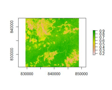
The resulting NDVI can be viewed in the above figure. As expected the NDVI ranges from about 0.2, which corresponds to nearly bare soils, to 0.9 which means that there is some dense vegetation in the area.
Although this is a quick way to perform the calculation, directly adding, subtracting, multiplying, etc, the layers of big raster objects is not recommended. When working with big objects, it is advisable to use the calc() function to perform these types of calculations. The reason is that R needs to load all the data first into its internal memory before performing the calculation and then running everything in one block. It is really easy to run out of memory when doing that. A big advantage of the calc() function is that it has a built-in block processing option for any vectorized function, allowing such calculations to be fully "RAM friendly". The example below illustrates how to calculate NDVI from the same data set using the calc() function.
## Define the function to calculate NDVI from
ndvCalc <- function(x) {
 ndvi <- (x\[\[4\]\] - x\[\[3\]\]) / (x\[\[4\]\] + x\[\[3\]\])
 return(ndvi)
}
ndvi2 <- calc(x=gewata, fun=ndvCalc)
Note that overlay() can also be used in that case to obtain the same result, with the same level of RAM friendliness. The advantage of overlay() is that the number of input RasterLayers is less limiting. As a consequence specifying the layers does not happen in the function call but in the overlay() call instead.
ndvOver <- function(x, y) {
 ndvi <- (y - x) / (x + y)
 return(ndvi)
}
ndvi3 <- overlay(x=gewata\[\[3\]\], y=gewata\[\[4\]\], fun=ndvOver)
We can verify that the three layers ndvi, ndvi2, and ndvi3 are identical using the all.equal() function from the raster package.
all.equal(ndvi, ndvi2)
## \[1\] TRUE
all.equal(ndvi, ndvi3)
## \[1\] TRUE
In the simple case of calculating NDVI, we were easily able to produce the same result with calc() and overlay(), however, it is often the case that one function is preferable to the other. As a general rule, a calculation that needs to refer to multiple individual layers separately will be easier to set up in overlay() than in calc().
Re-projections
By the way, we still don't know where this area is. In order to investigate that, we are going to try projecting it on Google Earth. As you know Google Earth is all in Lat/Long, so we have to get our data re-projected to Lat/Long first. The projectRaster() function allows re-projection of raster objects to any projection one can think of. As the function uses the PROJ.4 library (the reference library, external to R, that handles cartographic projections and performs projections transformations; the rgdal package is the interface between that library and R) to perform that operation, the crs= argument should receive a PROJ.4 expression. PROJ.4 expressions are strings that provide the projection parameters of cartographic projections. A central place to search for projections is the spatial reference website http://spatialreference.org/, from this database you will be able to query almost any reference and retrieve it in any format, including its PROJ.4 expression.
## One single line is sufficient to project any raster to any projection
ndviLL <- projectRaster(ndvi, crs='+proj=longlat')
Note that if re-projecting and mosaicing is a substantial part of your project, you may want to consider using the gdalwarp command line utility (gdalwarp) directly. The gdalUtils R package provides utilities to run GDAL commands from R, including gdalwarp, for re-projection, resampling, and mosaicing.
Now that we have our NDVI layer in Lat/Long, let's write it to a KML file, which is one of the two Google Earth formats.
# Since this function will write a file to your working directory
# you want to make sure that it is set where you want the file to be written
# It can be changed using setwd()
getwd()
# Note that we are using the filename argument, contained in the ellipsis (...) of
# the function, since we want to write the output directly to file.
KML(x=ndviLL, filename='gewataNDVI.kml')
Note that you need to have Google Earth installed on your system to perform the following step. Now let's find that file that we have just written and double-click it, and watch how Google Earth brings us all the way to ... Ethiopia. More information will come later in the course about that specific area.
We are done with this data set for this lesson. So let's explore another data set, from the Landsat sensors. This dataset will allow us to find other interesting raster operations to perform.
More raster arithmetics: performing simple value replacements
Since 2014, the USGS has started releasing Landsat data processed to surface reflectance. This means that they are taking care of important steps such as atmospheric correction and conversion from sensor radiance to reflectance factors. Additionally, they provide a cloud mask with this product. The cloud mask is an extra raster layer, at the same resolution as the surface reflectance bands, that contains information about the presence or absence of clouds as well as shadowing effects from the clouds. The cloud mask of Landsat surface reflectance product is named cfmask, after the name of the algorithm used to detect the clouds. For more information about cloud detection, see the algorithm page, and the publication by @zhu2012object. In the following section, we will use that cfmask layer to mask out the remaining clouds in a Landsat scene.
About the area
The area selected for this exercise covers most of the South Pacific island of Tahiti, French Polynesia. It is a mountainous, volcanic island, and according to Wikipedia, about 180,000 people live on the island. For convenience, the Landsat scene was subsetted to cover only the area of interest and is stored online.
## Download the data
download.file(url='../data/tahiti.zip', destfile='tahiti.zip', method='auto')
unzip(zipfile='tahiti.zip')
## Load the data as a RasterBrick object and investigate its content
tahiti <- brick('LE70530722000126_sub.grd')
tahiti
## Display names of each individual layer
names(tahiti)
## Visualize the data
plotRGB(tahiti, 3,4,5)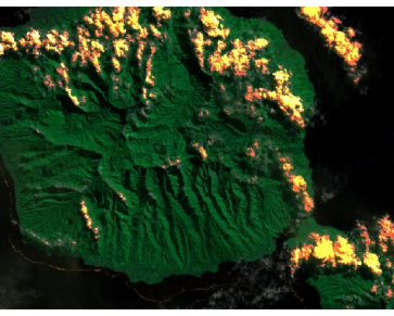
We can also visualize the cloud mask layer (layer 7).
plot(tahiti, 7)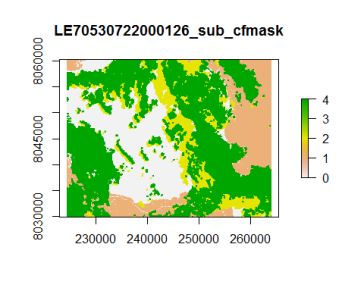
According to the algorithm description, water is coded as 1, cloud as 4, and cloud shadow as 2. Does the cloud mask fit with the visual interpretation of the RGB image we plotted before? We can also plot the two on top of each other, but before that, we need to assign no values (NA) to the 'clear land pixels' so that they appear transparent on the overlay plot.
## Extract cloud layer from the brick
cloud <- tahiti\[\[7\]\]
## Replace 'clear land' with 'NA'
cloud\[cloud == 0\] <- NA
## Plot the stack and the cloud mask on top of each other
plotRGB(tahiti, 3,4,5)
plot(cloud, add = TRUE, legend = FALSE)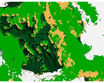
Applying a cloud mask to a dataset simply consists in performing value replacement. In this case, a condition on the 7th layer of the stack (the fmask layer) will determine whether values in the other layers are kept, or replaced by NA, which is equivalent to masking them. It is more convenient to work on the cloud mask as a separate RasterLayer, we will therefore split the RasterBrick using the dropLayer() function.
## Extract cloud mask RasterLayer
fmask <- tahiti\[\[7\]\]
## Remove fmask layer from the Landsat stack
tahiti6 <- dropLayer(tahiti, 7)
We will first do the masking using simple vector arithmetic as if tahiti6 and fmask were simple vectors. We want to keep any value with a 'clean land pixel' flag in the cloud mask; or rather, since we are assigning NAs, we want to discard any value of the stack which has a corresponding cloud mask pixel different from 0. This can be done in one line of code.
## Perform value replacement
tahiti6\[fmask != 0\] <- NA
However, this is possible here because both objects are relatively small and the values can all be loaded into the computer memory without any risk of overloading it. When working with very large raster objects, you will very likely run into problems if you do that. It is then preferable, as presented earlier in this tutorial to use calc() or overlay(). overlay() in this case is the appropriate function since we are working with two distinct raster objects.
## First define a value replacement function
cloud2NA <- function(x, y){
 x\[y != 0\] <- NA
 return(x)
}
The value replacement function takes two arguments, x and y. Similarly to what we did earlier, x corresponds to the RasterBrick, and y to the cloud mask.
# Let's create a new 6 layers object since tahiti6 has been masked already
tahiti6_2 <- dropLayer(tahiti, 7)
## Apply the function on the two raster objects using overlay
tahitiCloudFree <- overlay(x = tahiti6_2, y = fmask, fun = cloud2NA)
## Visualize the output
plotRGB(tahitiCloudFree, 3,4,5)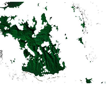
There are holes in the image, but at least the clouds are gone. We could use another image from another date, to create a composited image, but that is a little bit too much for today.
Summary
Today you got a general introduction to the raster package, its basic functions, its object classes, and methods. They can be categorized as follows:
Raster classes
RasterLayer: Single-layer object.RasterStackandRasterBrick: Multi-layer raster objects.
Functions
Read data
raster(): Read a single-layer raster object written on disk or read the first layer of a multi-layer object.brick(): Read a multi-layer raster object written on disk.
Write data
writeRaster(): Write aRasterLayer,RasterBrickorRasterStackto disk.filename = argument: available for most functions of the raster package that produce raster objects, write directly the output of the function to disk.
Reformat data
crop(): modify the extent of a Raster object based on another spatial object or an extent object.projectRaster(): Reproject (and resample) a raster object to a desired coordinate reference system.stack(): Assemble RasterLayers in a multilayer object.dropLayer(): Remove a layer from a multi-layer object (RasterStackorRasterBrick).
Simple visualization
plot(): Plot a raster object, usingadd = TRUEto overlay several objects.plotRGB(): Plot an RGB color composite
Raster calculations
- Raster objects work just like vectors of numerics (c(1,2,3)). They can be subsetted, added, subtracted, etc.
calc(): Apply a function to every pixel independently of a single raster object (Single or multi-layer). RAM friendly and can write output directly to disk using the filename = argument.overlay(): Apply a function that takes values from multiple raster objects. Similar tocalc()but for multiple objects.