Introduction
R is a statistical analysis software with wide capabilities. R's success is partially related to the growing number of tools and packages that are available to users.
If you haven't already, download RStudio, a set of integrated tools designed to help you be more productive with R. Find the proper version at the bottom of the page, download, and install it. Start R.
Installing Packages
We will be working with many packages. You will have the chance to learn how to download, install, and work with them.
- Open an R-script window by clicking on
File>New File> R-script. - The new window is where you would insert your R Script.
- Install packages using
install.packge(<PACKAGE_NAME>)
As a starter, we would like to install a few packages to work with Landsat Images. Since bfastSpatial package is still under development, you would need to install it directly from GitHub. Install devtools first. Then, use install_github to install bfastSpatial. The rest is very typical:
install.packages('devtools')
install_github('loicdtx/bfastSpatial')
You might get some errors because this package is still under development and many of its dependencies are not installed on your computer. If you get errors during the installation process, please read the error messages carefully. If you read the last few lines of the error message, it should inform you that a package is missing. Use your knowledge of package installation to resolve these issues. You might need to install as many as 4 additional packages, but R does not give you all 4 names at once. You should resolve the first error and attempt to install bfastspatial again. Then you would get another error. Install the second package and repeat the processes.
Install the following two packages as well:
install.packages("rgdal")
install.packages("raster")
Now, load the installed packages. R does not try to load all the libraries at once to save memory and time. Thus, if you need to work with a package, you would need to load it using the library() or require() functions.
require("devtools")
require("bfastSpatial")
require("rgdal")
require("raster")
require("tools")
R is case sensitive, uppercase and lowercase words and commands and functions are different from one another.
Set Working Directories
Like any programming task, you would benefit from setting working directories before getting busy with solving the problems. You will define the input and the output directories.
You are given some data to work with. Define the input and output directory for both the data and the shapefile.
Please check the below directories and change them to match the data directories on your computer.
You can either manually type in the path here, or, use the indir and outdir functions to get the data path directory with a copy/paste.
indir <- "PATH TO THE DATA"
outdir <- "PATH TO THE OUTPUT"
# PC example:
indir <- "C:/my/data/directory"
# Mac or Linux example:
indir <- "/my/data/directory"
dir.create(outdir, showWarning=FALSE)
crop_file<- "PATH TO THE SHAPEFILE CO5.shp"
Reading the Data
Processing raw Landsat imagery is fast and straightforward with R.
First, read your data into the R memory. Since we have more than one file in this example, we can first create a list of the files in the folder. Notice that you are creating an object, mylist, to refer to this list. The name of this object is almost arbitrary. But you would want to use names that are representative of the actual information "attached" to them.
Here we are working with gride files. The following syntax will find them for you.
Locate the tar files to be processed.
mylist <- list.files(indir, full.names=TRUE, pattern="\*.gz")
# for text files
mylist <- list.files(indir, full.names=TRUE, pattern="*.txt")
Getting help from R
R offers help regarding details of each package and function. The best way to prompt R for help is to type a ?followed by the function name. Let's try it for our next function using ?plot.
Data manipulation and extraction
Read the shapefile to crop the data to the desired extent. We call it Crop_obj (Crop Object) and it is the extent of the CO5 (Colorado 5) station.
crop_name <- file_path_sans_ext(basename(crop_file))
crop_obj <- readOGR(dsn=crop_file, crop_name, verbose=FALSE)
The first line returns the file path without the extension while basename omits everything but the file name.
A very important point about R - remember that each data layer you work with has a coordinate system. Refer to this link to read more about geographic coordinate systems. What you would like to do is to make sure that all layers in your data set have the same coordinate system. Use the projection function to check and see.
In this example, we have done this for you. But always make sure that both your rasters and shapefiles have the same coordinate system. Also, since you will be working on a specific area, you will be working with a set of imagery that have the same coordinate system, so no worries there.
Check the projection of your shapefile object. A print of the projection should output the following:
coord. ref. : +proj=utm +zone=13 +datum=WGS84 +units=m +no_defs +ellps=WGS84 +towgs84=0,0,0 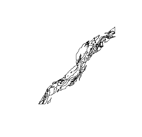
Generate (or extract, depending on whether the layer is already in the archive or not) NDVI for the first archived file. Notice that we are using the above shapefile to crop the Landsat image. We will only work with the area inside the crop object.
Also notice that a mask had to be selected; in that case, fmask, which is one of the layers of the Landsat archive file delivered by USGS/ESPA. For details about that mask and to know which values to keep (keep=), you can visit this page, or for general information on the layers provided in the archive, see the product guide.
Masking and cropping are optional but highly recommended if you intend to perform subsequent time-series analysis with the layers produced.
The extension of the output is by default .grd. This is the native format of the raster package. This format has many advantages over more common GeoTiff or ENVI formats.
processLandsat(x=mylist\[1\], vi='ndvi', outdir=outdir, srdir=outdir, delete=TRUE,
mask='fmask', keep=0, e=extent(crop_obj), overwrite=TRUE)srdir: Specify where the tarball should be uncompressed.delete: Toggle whether surface reflectance files (hdf/tiff) should be deleted after the vegetation index is calculated.
The result of the above function has produced nice sections of NDVI imagery for our study site. Let's plot that:
list <- list.files(outdir, pattern=glob2rx('\*.grd'), full.names=TRUE)
plot(r <- mask(raster(list\[1\]), crop_obj))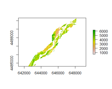
We use the raster function to visualize the data. The mask function crops the raster data to fit the shapefile specified.
Visualization of Multiple Landsat Scenes
Now we would like to attempt to visualize both layers and processes to perform a time series analysis.
Make a list of both of your output files.
list <- list.files(outdir, pattern=glob2rx('*.grd'), full.names=TRUE)
list
# [1] "C:/Users/itai/Documents/251C/Lab1/outputs/ndvi.LT50330322010117.grd"
# [2] "C:/Users/itai/Documents/251C/Lab1/outputs/ndvi.LT50330322010149.grd"
Now print the filenames and their location. This is just to check how many files we have in the system.
# "ndvi.LT50330322010117.grd"
# "ndvi.LT50330322010117.gri"
# "ndvi.LT50330322010149.grd"
# "ndvi.LT50330322010149.gri"
# Located in "C:/Users/itai/Documents/251C/Lab1/outputs"
You tell the dates of the files listed in your out directory by looking at the filename.
Creating a multi-temporal raster object
Create a new sub-directory to store the raster stack
outdir2 <- paste0(outdir, "/", "stack_new")
dir.create(outdir2, showWarnings=FALSE)
The paste0 function concatenates vectors after converting to characters, with zero-length arguments being recycled to a string with no value, i.e. "".
Generate a file name for the output stack:
stackName <- file.path(outdir2, 'CO5_Stack.grd')Stack the layers. Once the vegetation index layers have been produced for several dates, they can be stacked, to create a multilayer raster object, with time dimension written in the file as well. The function to perform this operation on Landsat data is the timeStack. By simply providing a list of file names or a directory containing the files, the function will create a multilayer object and directly parse through the file names to extract temporal information from them and write that information to the object created.
s <- timeStack(x=list, filename=stackName, datatype='INT2S', overwrite=TRUE)
## Visualize both layers
plot(s)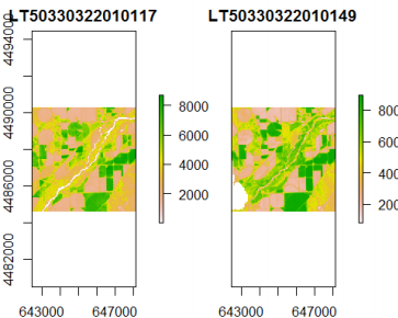
Processed to mask out the unwanted regions using the crop_obj.
plot(mask(s, crop_obj))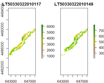
Looking at the bottom-left of the above two images, they are different because there is a cloud blocking the satellite imagery.
The image on the right is also "greener" than the one in the left. The NDVI is found using the formula of near-infrared radiation minus visible radiation divided by near-infrared radiation plus visible radiation. An increase in vegetation and chlorophyll would result in more visible light being absorbed by the plants and therefore a darker green.
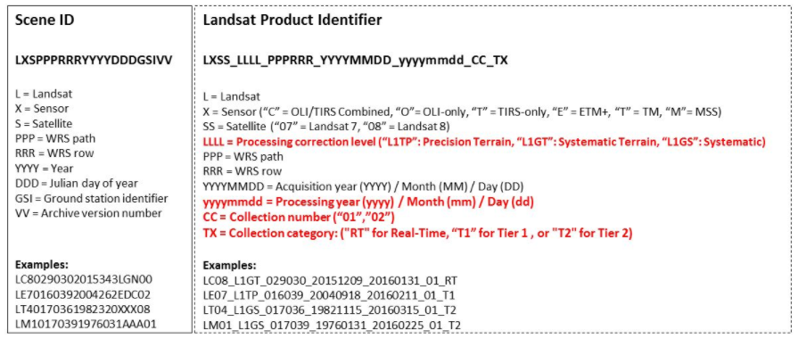
The Landsat filename provides the user with information on the satellite that collected the data. The Landsat filename can be read as L_T_5_033_032_2010_149, with
- L = Landsat
- T = Sensor (TIRS-only)
- 5 = Satellite
- 033 = WRS path
- 032 = WRS row
- 2010 = Year
- 149 = day of the year (May 29th)
See the image below for filename convention.
About the example above
- For this function to work, it is absolutely necessary that the input layers have the same extent. Two Landsat scenes belonging to the same path/row, but acquired at different times often have slightly different extents. We, therefore, recommend always using an extent object in processing Landsat, even when working with full scenes.
- Time information is automatically extracted from the layer names (using
getSceneInfo) and written to the z dimension of the stack. - We chose to write the output to the .grd format, which allows the time information to be stored as well as the original layer names.
- The x= argument can also simply be the directory containing the layers; in which case we recommend using pattern= as well to ensure that only the desired files are included.