Introduction
The information here, about handling HDF4 format files with R is additional to the lesson content, however, it will be useful for you in the future; particularly if you plan to work with MODIS data
Packages you should know about
The gdalUtils package provides interesting wrappers facilitating the use of GDAL functions from within R.
Exercise: Design a pre-processing chain to assess change in NDVI over time
I would like to know if Wageningen, Netherlands, and its surroundings have changed with respect to its spring NDVI over the past 15 years. For that, I would need to do a bi-temporal comparison of two NDVI images, acquired in spring. Simply subtracting the images should work, but unfortunately, these haven't been pre-processed yet. I managed to download two Landsat raw surface reflectance products covering the area. They were acquired around the same period of the year, but about 30 years apart from each other. I don't know how to compare them.
Can you please help me?
Data is available at: </data/Wageningen.zip> Note: Landsat 8 does not use the same band numbers as its predecessors. Red and NIR correspond to band3 and band4 respectively for ETM+ and TM (Landsat 7 and 5 respectively), while for OLI (Landsat 8), Red is band4 and NIR is band5.
Hints
list.files()with pattern = argument. For example,list.files('data/', pattern = glob2rx('\*.tif'), full.names = TRUE)will return only the files that have the.tifextension.- You should always use
full.names = TRUEinlist.files()to be able to use the output directly. ?intersectuntar()to programmatically extract the files from the archive.
How to submit
Create a well-structured reproducible R project showing in the main R file:
- The workflow to pre-process the data
- Some visualization of the intermediary outputs
- How to produce and visualize the final output
Introduction to Vector with R
Objective of today
- Learn how to handle vector data
Learning outcomes of today:
In today's lecture, we will explore the basics of handling spatial vector data in R. There are several R packages for this purpose but we will focus on using sp, rgdal, rgeos, and some related packages. At the end of the lecture, you should be able to:
- create point, line, and polygon objects from scratch;
- explore the structure of sp classes for spatial vector data;
- plot spatial vector data;
- transform between datums and map projections;
- apply basic operations on vector data, such as buffering, intersection and area calculation;
- write spatial vector data to a
kmlfile;
Vector R Basics
Some packages for working with spatial vector data in R
The packages sp and rgdal are widely used throughout this course. Both packages not only provide functionality for raster data but also vector data.
The sp package provides classes for importing, manipulating, and exporting spatial data in R, and methods for doing so. It is often the foundation for other spatial packages, such as raster. The rgdal package includes bindings to parts of the OGR Simple Feature Library which provides access to a variety of vector file formats such as ESRI Shapefiles and kml. The OGR library is part of the widely used Geospatial Data Abstraction Library (GDAL). The GDAL library is the most useful freely-available library for reading and writing geospatial data. The GDAL library is well-documented (http://gdal.org/), but with a catch for R and Python programmers. The GDAL (and associated OGR) library and command line tools are all written in C and C++. Bindings are available that allow access from a variety of other languages including R and Python but the documentation is all written for the C++ version of the libraries. This can make reading the documentation rather challenging. Fortunately, the rgdal package, providing GDAL bindings in R, is also well documented with lots of examples. The same is valid for the Python libraries.
Similarly, rgeos is an interface to the powerful Geometry Engine Open Source (GEOS) library for all kinds of operations on geometries (buffering, overlaying, area calculations, etc.). Thus, functionality that you commonly find in expensive GIS software is also available within R, using free but very powerful software libraries.
The possibilities are huge. In this course, we can only scratch the surface with some essentials, which hopefully invite you to experiment further and use them in your research. Details can be found in the book Applied Spatial Data Analysis with R and several vignettes authored by Roger Bivand, Edzer Pebesma, and Virgilio Gomez-Rubio. Owing to time constraints, this lecture cannot cover the related package spacetime with classes and methods for spatio-temporal data.
Creating and manipulating geometries
The package sp provides classes for spatial-only geometries, such as SpatialPoints (for points), and combinations of geometries and attribute data, such as a SpatialPointsDataFrame. The following data classes are available for spatial vector data:
Overview of sp package spatial-only geometry classes.
| Geometry | class | attribute |
|---|---|---|
| points | SpatialPoints | No |
| points | SpatialPointsDataFrame | data.frame |
| line | Line | No |
| lines | Lines | No |
| lines | SpatialLines | No |
| lines | SpatialLinesDataFrame | data.frame |
| rings | Polygon | No |
| rings | Polygons | No |
| rings | SpatialPolygons | No |
| rings | SpatialPolygonsDataFrame | data.frame |
We will go through a few examples of creating geometries from scratch to familiarize ourselves with these classes.
First, start Google Earth on your computer and make a note of the longitude and latitude of two points in Los Angeles that are relevant to you. Use a decimal degree notation with at least 4 digits after the decimal point. To change the settings in Google Earth click 'Tools | Options' and change the Show Lat/Long setting on the 3D View Tab.
Points: SpatialPoints, SpatialPointsDataFrame
The example below shows how you can create spatial point objects from these coordinates. Type ?function name (e.g. ?cbind) for finding help on the functions used.
Class "CRS" of coordinate reference system arguments. Interface class to the PROJ.4 projection system. The class is defined as an empty stub accepting the value NA in the sp package. If the rgdal package is available, then the class will permit spatial data to be associated with coordinate reference systems.
## Load the sp and rgdal packages
library(sp)
library(rgdal)

## Coordinates of two points identified in Google Earth, for example: pnt1_xy <- cbind(-118.465, 34.0463) # enter your own coordinates pnt2_xy <- cbind(-118.472, 34.062) # enter your own coordinates

## Combine coordinates in single matrix
coords <- rbind(pnt1_xy, pnt2_xy)

## Make spatial points object
prj_string_WGS <- CRS("+proj=longlat +datum=WGS84")
mypoints <- SpatialPoints(coords, proj4string=prj_string_WGS)

## Inspect object
class(mypoints)
str(mypoints)

## Create and display some attribute data and store in a data frame
mydata <- data.frame(cbind(id = c(1,2)
 Name = c("my first point",
 "my second point")))

## Make spatial points data frame
mypointsdf <- SpatialPointsDataFrame(
 coords, data = mydata,
 proj4string=prj_string_WGS)
class(mypointsdf) # Inspect and plot object
names(mypointsdf)
str(mypointsdf)

spplot(mypointsdf, zcol="Name", col.regions = c("red", "blue"), xlim = bbox[mypointsdf](1, )\]+c(-0.01,0.01),
 ylim = bbox[mypointsdf](2, )\]+c(-0.01,0.01),
 scales= list(draw = TRUE))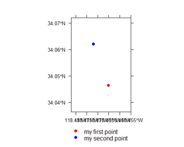
Play with the spplot function
What is needed to make the following work?
spplot(mypointsdf, col.regions = c(1,2))The difference between the objects mypoints and mypointsdf is that mypoints is a spatial points object, while mypointsdf is a spatial point data frame.
Lines
Now let us connect the two points by a straight line. First, find information on the classes for lines that are available in sp. The goal is to create SpatialLinesDataFrame but we have to go through some other classes.
## Consult help on SpatialLines class
(simple_line <- Line(coords))
## An object of class "Line"
## Slot "coords"
## \[,1\] \[,2\]
## \[1,\] -118.465 34.0463
## \[2,\] -118.472 34.0620
(lines_obj <- Lines(list(simple_line), "1"))
## An object of class "Lines"
## Slot "Lines"
## \[\[1\]\]
## An object of class "Line"
## Slot "coords"
## \[,1\] \[,2\]
## \[1,\] -118.465 34.0463
## \[2,\] -118.472 34.0620
##
##
##
## Slot "ID"
## \[1\] "1"
(spatlines <- SpatialLines(list(lines_obj), proj4string=prj_string_WGS))
## An object of class "SpatialLines"
## Slot "lines"
## \[\[1\]\]
## An object of class "Lines"
## Slot "Lines"
## \[\[1\]\]
## An object of class "Line"
## Slot "coords"
## \[,1\] \[,2\]
## \[1,\] -118.465 34.0463
## \[2,\] -118.472 34.0620
##
##
##
## Slot "ID"
## \[1\] "1"
##
##
##
## Slot "bbox"
## min max
## x -118.4720 -118.465
## y 34.0463 34.062
##
## Slot "proj4string"
## CRS arguments
## +proj=longlat +datum=WGS84 +ellps=WGS84 +towgs84=0,0,0 (line_data <- data.frame(Name = "straight line", row.names="1"))
## Name
## 1 straight line
(mylinesdf <- SpatialLinesDataFrame(spatlines, line_data))
## An object of class "SpatialLinesDataFrame" ## Slot "data"
## Name
## 1 straight line
##
## Slot "lines"
## \[\[1\]\]
## An object of class "Lines"
## Slot "Lines"
## \[\[1\]\]
## An object of class "Line"
## Slot "coords"
## \[,1\] \[,2\]
## \[1,\] -118.465 34.0463
## \[2,\] -118.472 34.0620
##
##
##
## Slot "ID"
## \[1\] "1"
##
##
##
## Slot "bbox"
## min max
## x -118.4720 -118.465
## y 34.0463 34.062
##
## Slot "proj4string"
## CRS arguments
## +proj=longlat +datum=WGS84 +ellps=WGS84 +towgs84=0,0,0 Question 3: What is the difference between Line and Lines?
class(mylinesdf)
str(mylinesdf)
spplot(mylinesdf, col.regions = "blue",
 xlim = bbox[mypointsdf](1, )\]+c(-0.01,0.01), ylim = bb[mypointsdf](2, ), \]+c(-0.01,0.01), scales= list(draw = TRUE))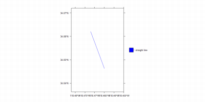
Try to understand the above code and its results by studying help. Try to add the points together with the lines on the same map.
Writing and reading spatial vector data using OGR
What now follows is a brief intermezzo before we continue with the classes for polygons. Let us first export the objects created as KML files that can be displayed on Google Earth. We will use the OGR functionality available through the package rgdal.
library(rgdal)
## Write to KML; below we assume a subdirectory data within the current
# working directory
dir.create("data", showWarnings = FALSE)
writeOGR(mypointsdf, file.path("data","mypointsGE.kml"),
 "mypointsGE", driver="KML", overwrite_layer=TRUE)
writeOGR(mylinesdf, file.path("data","mylinesGE.kml"),
 "mylinesGE", driver="KML", overwrite_layer=TRUE)
Check (in Google Earth) whether the attribute data were written to the KML output.
The function readOGR allows the reading of OGR compatible data into a suitable spatial vector object. Similar to writeOGR, the function requires entries for the arguments dsn (data source name) and layer (layer name). The interpretation of these entries varies by driver. Please study the details in the help file.
Digitize a path (e.g. a bicycle route) between the two points of interest you selected earlier in Google Earth. This can be achieved using the Add Path functionality of Google Earth (see here for more info). Save the path in the data folder within the working directory under the name route.kml. We will read this file into a spatial lines object and add it to the already existing SpatialLinesDataFrame object.
dsn = file.path("data","route.kml")
ogrListLayers(dsn) # To find out what the layers are
myroute <- readOGR(dsn, layer = ogrListLayers(dsn))
## Put both in single data frame
proj4string(myroute) <- prj_string_WGS
## Warning in \`proj4string<-\`(\`\*tmp\*\`, value = <S4 object of class structure("C RS", package = "sp")>): A new CRS was assigned to an object with an existing CR S
## +proj=longlat +ellps=WGS84 +towgs84=0,0,0,0,0,0,0 +no_defs
## without reprojecting
## For reprojection, use function spTransform
names(myroute)
## \[1\] "Name" "Description"
myroute$Description <- NULL # delete Description
# mylinesdf <- rbind(mylinesdf, myroute)
# Note: some problems were reported with this step, see Q&A
mylinesdf <- rbind.SpatialLines(mylinesdf, myroute)
Try to understand the above code and results. Feel free to display the data and export it to Google Earth.
Transformation of Coordinate System
Transformations between coordinate systems are crucial to many GIS applications. The Keyhole Markup Language (kml) used by Google Earth uses latitude and longitude in a polar WGS84 coordinate system (i.e. geographic coordinates). However, in some of the examples below, we will use metric distances (i.e. cartographic coordinates). There are two types of coordinate systems that you need to recognize: projected coordinate systems and un-projected coordinates systems
One of the challenges of working with geospatial data is that geodetic locations (points on the Earth's surface) are mapped into a two-dimensional cartesian plane using a cartographic projection. Projected coordinates are coordinates that refer to a point on a two-dimensional map that represents the surface of the Earth (i.e. projected coordinate system). Latitude and Longitude values are an example of an un-projected coordinate system. These are coordinates that directly refer to a point on the Earth's surface. One way to deal with this is by transforming the data into a planar coordinate system. In R this can be achieved via bindings to the PROJ.4 - Cartographic Projections Library (http://trac.osgeo.org/proj/), which is available in rgdal. Central to spatial data in the sp package is that they have a coordinate reference system, which is coded in an object of CRS class. Central to operations on different spatial data sets is that their coordinate reference system is compatible (i.e., identical). This CRS can be a character string describing a reference system in a way understood by the PROJ.4 projection library, or a (character) missing value. An interface to the PROJ.4 library is available only if the R package rgdal is present.
We will transform our spatial data to the California State Plane Zone 5 (Zone V).
Please note that some widely spread definitions of the California State Plane grid (EPSG: 102245) are incomplete (see e.g. http://www.spatialreference.org and search for the EPSG number); - The PROJ.4 details can be found here: http://spatialreference.org/ref/esri/102245/
## Define CRS object for UTM projection
prj_string_UTM <- CRS("+proj=lcc +lat_1=34.03333333333333 +lat_2=35.46666666666 667 +lat_0=33.5 +lon_0=-118 +x_0=2000000 +y_0=500000 +ellps=GRS80 +units=m +no_ defs")
## Perform the coordinate transformation from WGS84 to UTM
mylinesUTM <- spTransform(mylinesdf, prj_string_UTM)
You can always plot the line using the basic plot command:
plot(mylinesUTM, col = c("red", "blue"))
box()
Now that the geometries are projected to a planar coordinate system, the length can be computed using a function from the package rgeos.
## Use rgeos for computing the length of lines
library(rgeos)
## rgeos version: 0.3-20, (SVN revision 535)
## GEOS runtime version: 3.5.0-CAPI-1.9.0 r4084
## Linking to sp version: 1.2-3
## Polygon checking: TRUE
(mylinesdf$length <- gLength(mylinesUTM, byid=T))
## 1 0
## 1857.542 3364.146
Feel free to export the updated lines to Google Earth or to inspect the contents of the data slot of the object mylinesdf:
mylinesdf@data
# or
data.frame(mylinesdf)
Polygons
Polygons with the sp package
We now continue with sp classes for polygon objects. The idea is to illustrate the classes; the data are meaningless. Let us create overlapping circles around the points you defined earlier.
## Perform the coordinate transformation from WGS84 (i.e. not a projection) to California State Plane (projected)"

# This step is necessary to be able to measure objectives in 2D (e.g. meters) (mypointsUTM <- spTransform(mypointsdf, prj_string_UTM))

## coordinates id Name
## 1 (1957065, 560698.2) 1 my first point
## 2 (1956427, 562442.7) 2 my second point
pnt1_UTM <- coordinates[mypointsUTM](1,)\]
pnt2_UTM <- coordinates[mypointsUTM](2,)\]
## Make circles around points, with radius equal to distance between points
## Define a series of angles going from 0 to 2pi
ang <- pi\*0:200/100
circle1x <- pnt1_UTM\[1\] + cos(ang) \* mylinesdf$length\[1\]
circle1y <- pnt1_UTM\[2\] + sin(ang) \* mylinesdf$length\[1\]
circle2x <- pnt2_UTM\[1\] + cos(ang) \* mylinesdf$length\[1\]
circle2y <- pnt2_UTM\[2\] + sin(ang) \* mylinesdf$length\[1\]
c1 <- cbind(circle1x, circle1y)
c2 <- cbind(circle2x, circle2y)
You can plot everything again using basic R plot commands:
plot(c2, pch = 19, cex = 0.2, col = "red", ylim = range(circle1y, circle2y), xl im = range(circle1x, circle2x))
points(c1, pch = 19, cex = 0.2, col = "blue")
points(mypointsUTM, pch = 3, col= "darkgreen")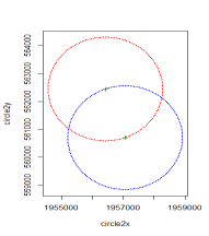
Now, we create subsequently
- Polygons
- SpatialPolygons
- SpatialPolygonsDataFrame
## Iterate through some steps to create SpatialPolygonsDataFrame object circle1 <- Polygons(list(Polygon(cbind(circle1x, circle1y))),"1") circle2 <- Polygons(list(Polygon(cbind(circle2x, circle2y))),"2") spcircles <- SpatialPolygons(list(circle1, circle2), proj4string=prj_string_UTM )
circledat <- data.frame(mypointsUTM@data, row.names=c("1", "2")) circlesdf <- SpatialPolygonsDataFrame(spcircles, circledat)
Similar results can be obtained using the function gBuffer of the package rgeos, as demonstrated below. Notice the use of two overlay functions from the package rgeos.
The final results can be plotted using basic R plotting commands:
plot(circlesdf, col = c("gray60", "gray40"))
plot(mypointsUTM, add = TRUE, col="red", pch=19, cex=1.5)
plot(mylinesUTM, add = TRUE, col = c("green", "yellow"), lwd=1.5)
box()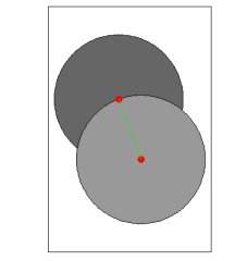
Here is an example of a plot of the results which employs a few more advanced options of spplot.
spplot(circlesdf, zcol="Name", col.regions=c("gray60", "gray40"), sp.layout=list(list("sp.points", mypointsUTM, col="red", pch=19, cex=1.5 ), list("sp.lines", mylinesUTM, lwd=1.5))) 
Try to understand how spplot works by breaking it down into simple steps e.g. spplot(circlesdf, zcol="Name", col.regions=c("gray60", "gray40"))
## Polygon Operations with rgeos (buffer, intersect, difference)
library(rgeos)
## Expand the given geometry to include the area within the specified width wit h specific styling options
buffpoint <- gBuffer(mypointsUTM\[1,\], width=mylinesdf$length\[1\], quadsegs=2) mydiff <- gDifference(circlesdf\[1,\], buffpoint)
plot(circlesdf\[1,\], col = "red")
plot(buffpoint, add = TRUE, lty = 3, lwd = 2, col = "blue")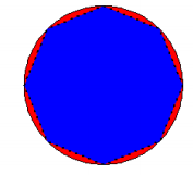
gArea(mydiff)
## what is the area of the difference?
## \[1\] 1078783
plot(mydiff, col = "red")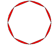
myintersection <- gIntersection(circlesdf\[1,\], buffpoint)
plot(myintersection, col="blue")
gArea(myintersection)
## \[1\] 9759380
print(paste("The difference in area =", round(100 \* gArea(mydiff) / gArea(myintersection),2), "%"))
## \[1\] "The difference in area = 11.05 %"
If you change quadsegs to a higher number, the better the approximation. Seeing as quadsegs: Number of line segments to use to approximate a quarter circle.
The difference between gIntersection and gDifference is as follows:
gIntersection: Function for determining the intersection between the two given geometries.gDifference: Function for determining the difference between the two given geometries.
Summary
We learned about:
- The spatial classes of the
sppackage - How to read/write data and change data format with
rgdalpackage (readOGR()andwriteOGR()) - Visualize spatial vector data in R and on Google Earth
- How to perform simple operations on Geometries in R using the
rgeospackage